我們前一篇關于人物識別跟蹤的文章《視頻連續目標跟蹤實現的兩種方法和示例(更新)》里講到，視頻圖像中物體的識別和跟蹤用到了卡爾曼濾波器(KF)。這里對這個話題我們稍微對這個卡爾曼濾波器進行一個整理。

目標跟蹤為什么用到卡爾曼濾波器(KF)?其實是因為我們假設了視頻的連續幀中的每個物體在圖像中的移動位置不會相差太多來進行的。我們在卡爾曼濾波器中設計了一個運動模式，這個運動模式可以讓我們估計在下一個圖像中每個被識別物體的所在位置，把每個位置和上一圖像中的位置進行比較統計，就可以定個七七八八了。

KF本質上是一種用于估計動態系統狀態的遞歸算法。它通過對系統的數學建模，輔以噪聲和不確定性假設，能夠從一系列不精確和噪聲污染的測量數據中推斷出系統的最優狀態估計。其核心思想是利用先驗知識和新獲得的測量信息來更新對系統狀態的估計，使得估計誤差最小化。誤差、噪聲干擾，這些設定符合我們實際應用場景中的所能得到的條件。而只有當信噪比足夠高，或者誤差幾乎可以忽略不計，并且構建的系統數學模型足夠準確時，才可以對測量計算得到的結果抱有信心，否則我們就需要在不完美的現實數據中，進行綜合

KF廣泛用于各種應用場景，特別是在需要高精度和實時處理的領域，如導航系統、自動駕駛技術、信號處理和控制系統等。

卡爾曼濾波器有多種類型，小編這里將只圍繞標準卡爾曼濾波器(KF)和擴展卡爾曼濾波器(Extended KF - EKF)講一點特性。

經典卡爾曼濾波器(KF)：

特點：適用于線性系統假設的隨機信號處理。包含兩步：預測和更新，每步都使用線性方程。

應用：常用于導航、控制系統及金融工程中

擴展卡爾曼濾波器(EKF)：

特點：擴展了標準KF，將其概念應用到非線性系統中。通過對非線性方程進行線性化處理，使用雅可比矩陣來估計狀態。簡單地講，就是把分線性方程在每個取值點處進行泰勒展開

應用：常用于非線性系統中，如機器人定位、航空航天導航。

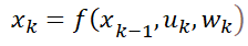
卡爾曼濾波器是一種用于估計動態系統狀態的最優遞歸算法，其核心基于以下兩組基本狀態方程模型：

	線性離散狀態空間方程	非線性離散狀態空間方程
過程方程

觀測方程

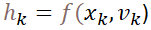KF對應的是上面的線性離散狀態方程，EKF對應的是上面的非線性離散狀態空間方程。

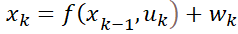
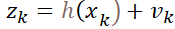
上面提到的非線性離散狀態空間方程中，噪聲特性是非加性噪聲。如果是加性噪聲，那么對應下面的公式：

????????（1）????????

????????（2）????????

但我們完全可以把這種加性噪聲作為非加性噪聲的一個特例處理。后面會提到并說明。

請記住這里的表示的系統狀態一般都是一個多維向量，所以我們這里討論隨機狀態分布的噪聲w和v兩個隨機噪聲變量其實是期望值等于0，協方差矩陣分別為Q、R的正態分布的矩陣。其中：

：nx1狀態向量，包含系統在時間步 ( k ) 的狀態；

A是狀態轉移矩陣，定義了系統的狀態如何從一個時間步轉移到下一個時間步；

u是px1控制輸入向量，描述了在時間步 ( k ) 作用于系統的外部控制輸入；

B是控制輸入矩陣，描述控制輸入如何影響狀態轉移；

是觀測向量，包含系統在時間步(k)的測量值或觀測值；

H是觀測矩陣，將系統狀態映射到觀測空間；

w通常假設為均值為零的高斯噪聲，影響狀態轉移；

v通常假設為均值為零的高斯噪聲，影響觀測；

f(x,u)，狀態轉移函數，描述系統狀態如何通過非線性函數從一個時間步轉移到下一個時間步；

h(x)，控制輸入函數，用于描述控制輸入如何與系統狀態通過非線性函數關聯。

對于正態分布的信號，經過線性變換之后對應的信號仍然符合正態分布；而經過非線性變換之后的非加性噪聲，一般就失去了正態分布的特性。示例如下：

一個正態分布的信號x~N(0, 1)，分別經過:

經 Y = 3x + 3 轉換或者映射之后，在0點的x取值是正態分布的情況下，線性變換后的Y仍然是符合正態分布，不過期望值=3，而Y的信號的方差變成了9。

E[Y] = E[3x+3] =E[3x] + 3 =3E[x] + 3 = 3*0 + 3 = 3

D[Y]=E{[Y - E(Y)]^2} =E{[3x+3 - 3]^2} =E[9x^2] =9E[x^2]=9

經Z = sin(x) 非線性轉換后，雖然其期望值（均值）仍然為0，但是分布不再符合正態分布的特性。

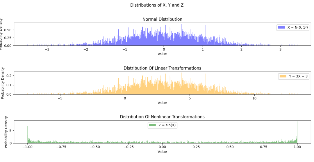
[圖-1]正態分布經過不同變換前后得到的分布比較

大家可以用下面的代碼用不同的轉換進行正態分布經歷不同的轉換后的分布模擬。

import numpy as np
import matplotlib.pyplot as plt


# Parameters for the normal distribution
mu_x = 0      # Mean of X
sigma_x = 1   # Standard deviation of X


# Linear transformation parameters
a = 3         # Scale factor
b = 3         # Shift factor


# Generate random samples from the normal distribution (X)
x = np.random.normal(mu_x, sigma_x, 5000)


# Apply the linear and nonlinear transformations
y = a * x + b
z = np.sin(x)


# 假設 x, y, z 是你的數據，mu_x, sigma_x, a, b 是參數。


# 設置子圖
fig, axes = plt.subplots(3, 1, figsize=(15, 5))  # 1 行，3 列


# 在第一個子圖中繪制 X 的直方圖
axes[0].hist(x, bins=1000, density=True, alpha=0.5, color='blue', label=f'X ~ N({mu_x}, {sigma_x}2)')
axes[0].set_xlabel('X')
axes[0].set_ylabel('Density')
axes[0].set_xlabel('Value')
axes[0].set_ylabel('Probability Density')
axes[0].set_title('Normal Distribution')
axes[0].legend()
# 在第二個子圖中繪制 Y 的直方圖
axes[1].hist(y, bins=1000, density=True, alpha=0.5, color='orange', label=f'Y = {a}X + {b}')
axes[1].set_xlabel('Y')
axes[1].set_ylabel('Density')
axes[1].set_xlabel('Value')
axes[1].set_ylabel('Probability Density')
axes[1].set_title('Distribution Of Linear Transformations')
axes[1].legend()
# 在第三個子圖中繪制 Z 的直方圖
axes[2].hist(z, bins=1000, density=True, alpha=0.5, color='green', label=r'Z = sin(X)')
axes[2].set_xlabel('Z')
axes[2].set_ylabel('Density')
axes[2].set_xlabel('Value')
axes[2].set_ylabel('Probability Density')
axes[2].set_title('Distribution Of Nonlinear Transformations')
axes[2].legend()
# 添加整體標題
plt.suptitle('Distributions of X, Y and Z')


# 顯示圖表
plt.tight_layout()
plt.show()

我們再回到EKF中，對于非線性系統的狀態方程，是通過對非線性系統的泰勒一次展開的方式在小區間內線性化推導（如我們在《紅外熱電堆的特性淺析及應用》中的對熱電堆內部結構熱傳遞的處理，以及《NTC測溫—查表計算vs公式計算》中局部的線性化處理等），然后得到的處理公式；而對于加性噪聲和非加性噪聲，在最后的遞歸處理步驟中，我們會看到不同的表達處理方式。
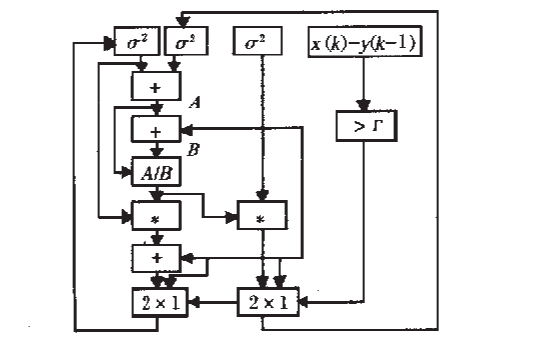
小編這里不對KF或者EKF最后的解算步驟進行推演，經常從卡爾曼濾波器中的兩個方程結果的示意圖中看到，KF解決的問題就是如何從兩種手段得到的系統狀態都是隨機數的情況下，如何來獲取更優結果。在收斂的情況下，我們通過KF或者EKF往往可以得到更優值。

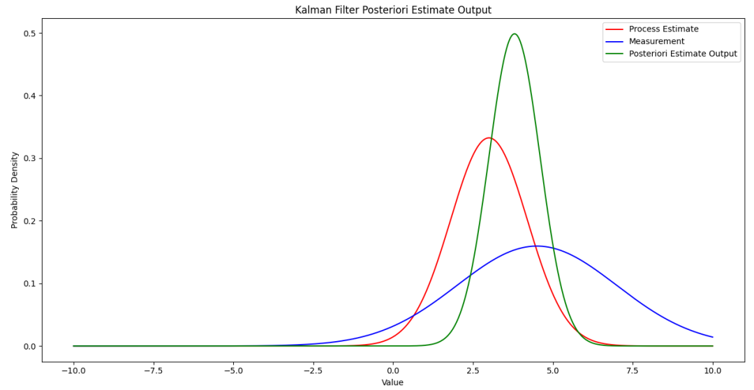
[圖-2]卡爾曼濾波器的狀態、測量和輸出噪聲分布

由于過程噪聲w~N(0,Q)和測量噪聲v~N(0,R)的存在，讓我們在根據模型得到的被噪聲干擾后的狀態隨機值和由傳感器或者其他數據采集設備得到的另外一組狀態隨機值之間需要做一個平衡后的輸出，最后的狀態值，也肯定會偏向在Q或者R中那個協方差更小的值。
有很多的書，網上也有很多的文章或者視頻介紹KF和EKF的推演的過程。有關文獻見本文參考部分。
必須要吐槽一下公眾號無法使用“圈”外的weblink，否則就直接上網頁鏈接，而不是拷貝鏈接了。

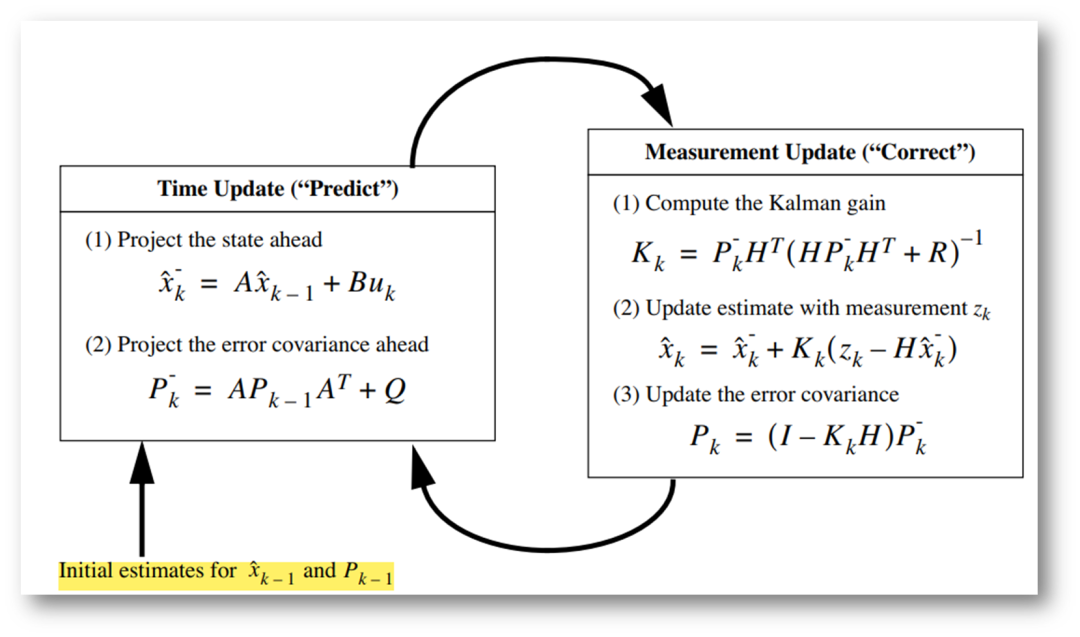
[圖-3]KF計算步驟[1][3]
在KF中，狀態轉移矩陣A，控制輸入向量u，控制輸入矩陣B，觀測矩陣H，測量向量Zk，過程噪聲協方差Q，測量噪聲協方差R，以及必要的后驗估計狀態值的初始值，后驗估計誤差協方差等都是已知的參數，就可以進行計算了：

從先驗估計值開始第一步計算；

然后計算后驗估計誤差協方差；

計算Kalman增益；

代入測量向量Zk和卡爾曼增益，得到后驗估計值(狀態的中間結果)；

迭代得到后驗估計誤差協方差，為下一次迭代準備。 ?

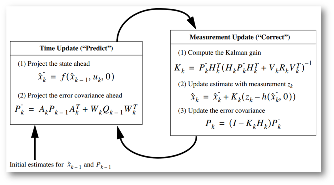
[圖-4]EKF的計算步驟(非加性噪聲)[1][2][3]

在上面的EKF計算步驟中，符號名稱很多還是一致的，但實際操作上存在一些差異。下面是它的操作步驟。

從先驗估計值開始第一步計算；

計算雅可比矩陣：

然后計算后驗估計誤差協方差；

計算Kalman增益，計算該增益前，包括以下兩個雅可比計算子項：

代入測量向量Zk和卡爾曼增益，得到后驗估計值(狀態的中間結果)；

迭代得到后驗估計誤差協方差，為下一次迭代準備。

如果是加性噪聲呢？我們再看前面的公式(1)和(2)，這時用下面的fA和hA來替代對應的公式：

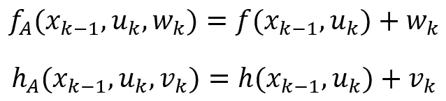
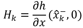
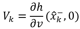
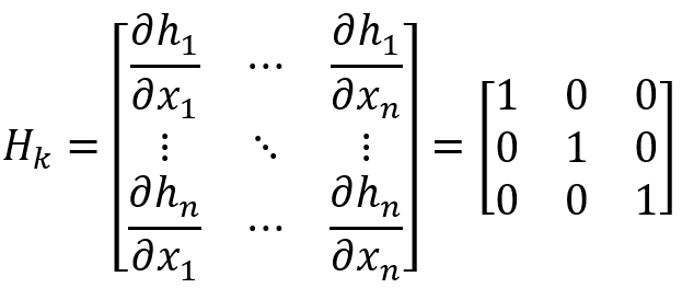
這種情況下，對和分別對w和v求偏導時候，得到的雅可比矩陣都是單位對角矩陣I，Wk和Vk就可以直接消掉了。 在EKF中，雅可比矩陣用于線性化非線性系統模型，并將其應用于狀態更新和測量更新的過程。例如下面狀態方程對狀態變量的偏導數。

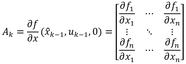
對于狀態更新，雅可比矩陣是系統狀態方程對狀態變量的偏導數，通常這個雅可比矩陣的維度是n×n，其中n是狀態變量的數量。

對于測量更新，雅可比矩陣是觀測方程對狀態變量的偏導數，其維度通常是m×n，其中m是測量變量的數量。如果m和n相等，那么這個情況下的雅可比矩陣也是方形的。

KF示例

在該示例中，我們用平拋物體的軌跡使用KF進行處理。按道理，因為存在1/2*g*t^2，這應該是一個非線性系統，能夠用狀態轉移矩陣(A)建立一個線性狀態模型，如x下面代碼所示，那么卡爾曼濾波器（KF）就足夠了。

卡爾曼濾波器適用于線性高斯狀態模型和觀測模型的情況。在示例的模型中，狀態轉移矩陣(A)是線性的，因為它具有固定的系數來描述位置、速度和加速度之間的關系，而沒有非線性項。如果你的測量模型（測量方程的矩陣）也是線性的，那么你可以直接使用標準的卡爾曼濾波器解決問題。

示例中，我們給定的初始條件：

x為水平方向，初始位置=0；

vx為水平速度方向，初始速度=3m/s:

x = v0 + vx * t；

y為垂直方向，初始位置和速度都是為0

y = y0 + vy0 * t +1/2 * g * t^2；

垂直方向只有加速度g，水平方向沒有阻力；

過程噪聲協方差Q賦值較小：

Q = np.eye(5) * 0.02 # Process noise covariance

Q[4,4] = 0 # 1g - gravity acceleration，穩定無噪聲

測量噪聲協方差R賦值稍大：

R = np.eye(2) * 1.5 # Measurement noise covariance

初始的后驗估計狀態誤差協方差P較大(我們要看一下收斂特性)：

P = np.eye(5) * 50

先看結果后看模擬代碼。為了彰顯KF的功能，把觀測狀態的協方差設置的稍微大了些，而把狀態轉移方程的誤差協方差設置得更小一些。可以看到幾乎發散的狀態的測量觀測值（紅線），KF的后驗狀態估計值都更靠近狀態轉移方程得到的數值。

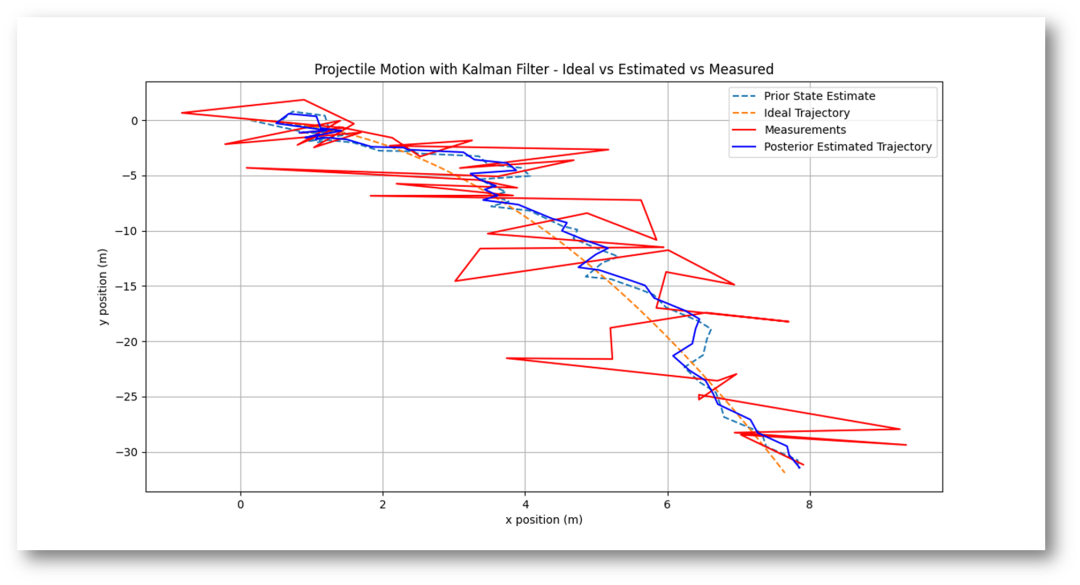
[圖-5]KF處理拋物線仿真（實藍線）

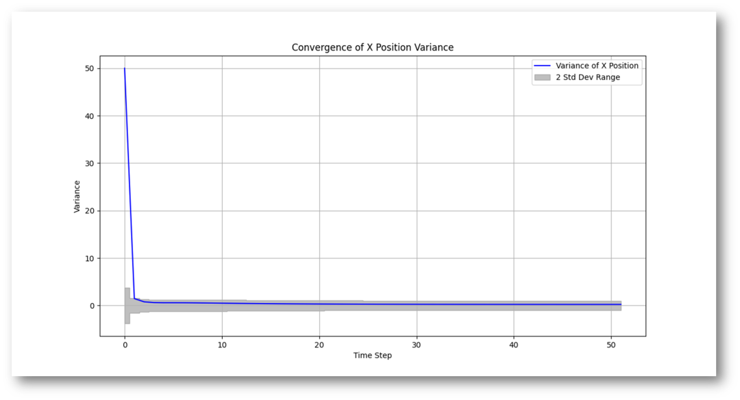
[圖-6]KF處理拋物線仿真x方向的位置后驗估計誤差協方差的收斂

特點說明：

盡管觀測測量的狀態亂七八糟，但是幸虧狀態轉移的模型足夠準確，讓最終的后驗狀態估計，那條實藍線，仍然可以繞在理論軌跡附近；

盡管后驗估計狀態誤差協方差P較大（50），但是KF處理過程中，我們可以看到該協方差以非常快的速度就收斂到了一個較小且穩定的數值。代碼中對標準差范圍取值有補充說明。圖-6中的灰色輪廓線只用到了+/-2σ的公差范圍。

拋物線KF模擬代碼：

import numpy as np
import matplotlib.pyplot as plt


# Define constants
dt = 0.05  # time interval
g = 9.81  # gravitational acceleration


# Initial state [x, vx, y, vy, ay]
initial_state = np.array([0, 3, 0, 0, -g])  # initial position (0,0) with vx0=3, vy0=0


# State transition matrix
F = np.array([[1, dt, 0, 0, 0],
              [0, 1, 0, 0, 0],
              [0, 0, 1, dt, 0.5 * dt**2],
              [0, 0, 0, 1, dt],
              [0, 0, 0, 0, 1]])


# Observation matrix
H = np.array([[1, 0, 0, 0, 0], 
              [0, 0, 1, 0, 0]])


# Process and measurement noise matrices
Q = np.eye(5) * 0.02    # Process noise covariance
Q[4,4] = 0              # 1g - gravity acceleration


R = np.eye(2) * 1.5     # Measurement noise covariance


# Initial estimation covariance matrix
P = np.eye(5) * 50


# Lists to store positions
posterior_state_estimate, ideal_positions, measurements = [], [], []
prior_state_estimate = []
# Time steps for simulation
n_steps = 51


# Initialize state variables
state = initial_state.copy()
ideal_state = initial_state.copy()


# 生成過程噪聲，可以使用 Q 的對角線元素生成
process_noise_variance = np.diag(Q)  # 假設是一個對角矩陣


# 用于存儲方差的列表
position_X_variances = []
position_X_variances.append(P[0, 0])
position_Y_variances = []
position_Y_variances.append(P[2, 2])


process_state = initial_state.copy()
z_state_measure = initial_state[[0, 2]]


for _ in range(n_steps):
    # 狀態空間方程得到的模擬數據
    process_noise = np.random.normal(0, process_noise_variance, size=state.shape)
    process_state = F @ process_state + process_noise


    # 模擬測量得到的狀態：measurement state
    z_state_measure = H @ process_state + np.random.normal(0, np.sqrt(R.diagonal()))


    # Prediction step
    process_noise = np.random.normal(0, process_noise_variance, size=state.shape)
    state = F @ state + process_noise
    P = F @ P @ F.T + Q


    prior_state_estimate.append((state[0], state[2]))
    # Assume we get some measurements (with noise)
    ideal_state = F @ ideal_state
    #z_state_measure = H @ ideal_state + np.random.normal(0, np.sqrt(R.diagonal()))


    # Kalman Gain
    S = H @ P @ H.T + R
    K = P @ H.T @ np.linalg.inv(S)


    # Update step
    y = z_state_measure - H @ state
    state += K @ y
    P = (np.eye(len(K)) - K @ H) @ P


    # 存儲 x，y 位置的方差
    position_X_variances.append(P[0, 0])
    position_Y_variances.append(P[2, 2])
    # Store the results
    posterior_state_estimate.append((state[0], state[2]))
    ideal_positions.append((ideal_state[0], ideal_state[2]))
    measurements.append((z_state_measure[0], z_state_measure[1]))


# Convert lists to numpy arrays
prior_state_estimate = np.array(prior_state_estimate)
posterior_state_estimate = np.array(posterior_state_estimate)
ideal_positions = np.array(ideal_positions)
measurements = np.array(measurements)


# Plot the results
plt.figure(figsize=(10, 6))
plt.plot(prior_state_estimate[:,0],prior_state_estimate[:,1], label = 'Prior State Estimate',linestyle='--')
plt.plot(ideal_positions[:, 0], ideal_positions[:, 1], label='Ideal Trajectory', linestyle='--')
#plt.scatter(measurements[:, 0], measurements[:, 1], c='orange', label='Measurements', marker='o')
plt.plot(measurements[:, 0], measurements[:, 1], c='red', label='Measurements', linestyle='-')
plt.plot(posterior_state_estimate[:, 0], posterior_state_estimate[:, 1], c='blue', label='Posterior Estimated Trajectory', linestyle='-')
plt.xlabel('x position (m)')
plt.ylabel('y position (m)')
plt.title('Projectile Motion with Kalman Filter - Ideal vs Estimated vs Measured')
plt.legend()
plt.grid()
plt.show()


# 繪制X位置的方差隨時間的變化
"""
1倍標準差（±1σ）：大約68.27%的數據落在一個標準差范圍內，即從分布平均值向左右各一個標準差。
2倍標準差（±2σ）：大約95.45%的數據落在兩個標準差范圍內，這一個常用的置信區域，許多統計分析中常被用于定義數據的正常范圍。
3倍標準差（±3σ）：大約99.73%的數據落在三個標準差范圍內，通常用于識別異常值或者極端值。
"""
time_steps = range(n_steps+1)
plt.figure(figsize=(10, 5))
plt.plot(time_steps, position_X_variances, label='Variance of X Position', color='blue')
# Calculate twice the standard deviation
twice_std_dev = 2 * np.sqrt(position_X_variances)
plt.fill_between(time_steps, 
                 0 - np.sqrt(twice_std_dev), 
                 0 + np.sqrt(twice_std_dev), 
                 color='gray', alpha=0.5, step='mid', label='2 Std Dev Range')
plt.xlabel('Time Step')
plt.ylabel('Variance')
plt.title('Convergence of X Position Variance')
plt.legend()
plt.grid(True)
plt.show()


# 繪制Y位置的方差隨時間的變化
plt.figure(figsize=(10, 5))
plt.plot(time_steps, position_Y_variances, label='Variance of Y Position', color='blue')
# Calculate twice the standard deviation
twice_std_dev = 2 * np.sqrt(position_Y_variances)
plt.fill_between(time_steps, 
                 0 - np.sqrt(twice_std_dev), 
                 0 + np.sqrt(twice_std_dev), 
                 color='gray', alpha=0.5, step='mid', label='2 Std Dev Range')
plt.xlabel('Time Step')
plt.ylabel('Variance')
plt.title('Convergence of Y Position Variance')
plt.legend()
plt.grid(True)
plt.show()

EKF示例

該示例中，模擬一輛小車始終以沿著其自身的中軸線用速度V行駛，而且小車整體還以固定的轉速轉動。我們以這個為前提對其行駛軌跡[x,y]和轉動角度進行跟蹤輸出。

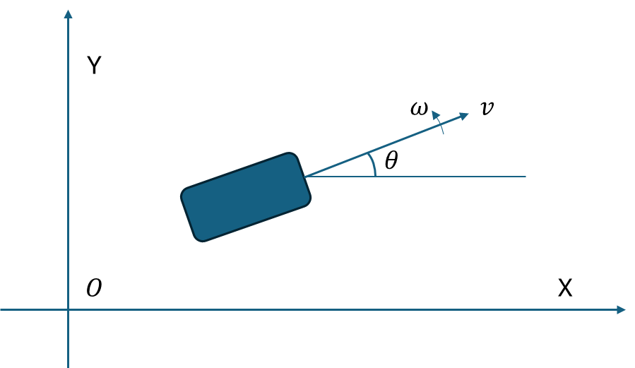
[圖-7]模擬小車的行駛和轉動

我們可以根據條件得到以下的狀態轉移方程(3)和觀測測量方程(4)：

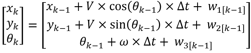
(3)

(4)

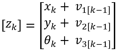
其中，w~N(0, Q)和v~[0, R]分別是過程噪聲和測量誤差噪聲。

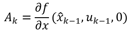
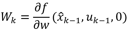
根據離散狀態方程，我們可以得到[圖-4]中的和：

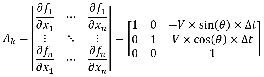
（5）

（6）

而[圖-4]中的Wk和Vk則是兩個單位矩陣。上面公式(5)和(6)需要留意代入的值。

先上圖后看代碼。仿真該小車逐漸轉彎的行駛軌跡和轉動角度的大小如下圖所示。

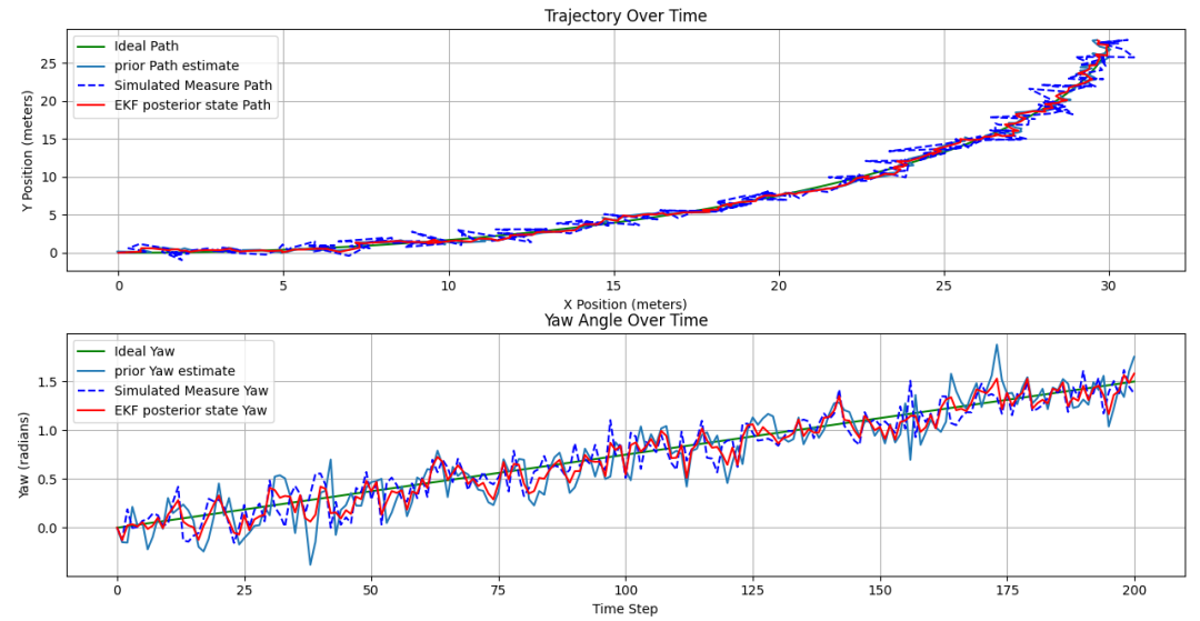
[圖-8]EKF模擬輸出的軌跡和轉動角度

如論如何，如果狀態方程和觀測方程的數值都不可靠，那么無論KF還是EKF，可能都將無法得到我們期望的結果。
EKF示例小車軌跡和轉角模擬代碼如下：

import numpy as np
import matplotlib.pyplot as plt


# A state space model for a differential drive mobile robot


# A matrix - 3x3 identity matrix
A_t_minus_1 = np.array([[1.0,  0,  0],
                        [  0,1.0,  0],
                        [  0,  0, 1.0]])


# Function to get the B matrix
def getB(yaw, dt):
    """
    Calculates and returns the B matrix
    3x2 matrix -> number of states x number of control inputs
    Expresses how the state of the system [x,y,yaw] changes
    due to the control commands
    :param yaw: The yaw angle in radians
    :param dt: The time change in seconds
    """
    B = np.array([[np.cos(yaw) * dt, 0],
                  [np.sin(yaw) * dt, 0],
                  [0, dt]])
    return B


# Define Jacobian for the transition function
def jacobian_of_motion(state, control, dt):
    _, _, yaw = state
    v, _ = control
    J_f = np.array([
        [1, 0, -v * np.sin(yaw) * dt],
        [0, 1, v * np.cos(yaw) * dt],
        [0, 0, 1]
    ])
    return J_f


def ekf_simulation(initial_state, control_vector, total_time, time_step):
    # Initialize state for EKF
    state_estimate = initial_state
    states_over_time = [state_estimate]


    # Simulated and ideal states tracking
    simulated_states = [initial_state]
    ideal_states = [initial_state]
    prior_states_estimate = [initial_state]
    
    # Initial posterior covariance of new estimate
    Pk = np.diag([1.0, 1.0, 1.0])


    # Measurement noise covariance matrix R_k
    # Measurement Noise init
    std_dev_x_mes = 0.5    # Standard deviation for x measurement
    std_dev_y_mes = 0.5    # Standard deviation for y measurement
    std_dev_yaw_mes = 0.15  # Standard deviation for yaw measurement
    
    R_k = np.diag([std_dev_x_mes**2, std_dev_y_mes**2, std_dev_yaw_mes**2])
    
    H = np.array([[1, 0, 0],
                  [0, 1, 0],
                  [0, 0, 1]])


    # Jacobian matrix J_h, which is the same as H for a linear model
    J_h = H
    
    # Process Noise init
    std_dev_x = 0.15
    std_dev_y = 0.15
    std_dev_yaw = 0.15


    # Simulation loop
    for _ in np.arange(0, total_time, time_step):
        # Ideal state (no noise)
        ideal_state = A_t_minus_1 @ ideal_states[-1] + getB(ideal_states[-1][2], time_step) @ control_vector
        ideal_states.append(ideal_state)


        # 1-1. State Prediction step
        # 生成過程噪聲
        process_noise_sim = np.random.normal(0, [std_dev_x, std_dev_y, std_dev_yaw], size=ideal_state.shape)


        Prior_state_Estimate = (A_t_minus_1 @ states_over_time[-1] + getB(states_over_time[-1][2], time_step) @ control_vector
                                + process_noise_sim)
        prior_states_estimate.append(Prior_state_Estimate)
        # 1-2. Process Error covariance
        Jf = jacobian_of_motion(states_over_time[-1], control_vector, dt=time_step)
        
        # Generate process noise for simulation as additive noise
        process_noise = np.random.normal(0, [std_dev_x, std_dev_y, std_dev_yaw])
        # Convert to a diagonal covariance matrix if needed for use in the EKF
        process_noise_cov = np.diag(process_noise**2)   
        
        Pk = Jf @ Pk @ Jf.T +  process_noise_cov #np.random.uniform(-process_noise, process_noise, 3)     
        
        # 2-1. Compute the Kalman gain
        K_k = Pk @  J_h.T @ np.linalg.inv(J_h @ Pk @ J_h.T + R_k)


        # Simulate sensor reading with measurement noise (using ideal_state)
        #tolerance_noise = np.random.uniform(-measurement_noise, measurement_noise, 3)
        measurement_noise = np.random.normal(0, [std_dev_x_mes, std_dev_y_mes, std_dev_yaw_mes])
        simulated_state = ideal_state + measurement_noise
        
        simulated_states.append(simulated_state)
        
        # 2-2. Update estimate with measurement z_k
        state_estimate = Prior_state_Estimate + K_k @ (simulated_state - J_h @ Prior_state_Estimate)
        
        # 2-3. Update the error covariance
        Pk = (np.eye(3) - K_k @ J_h) @ Pk


        # Record the updated state
        states_over_time.append(state_estimate)


    return np.array(prior_states_estimate), np.array(states_over_time), np.array(simulated_states), np.array(ideal_states)


def plot_states(prior_states_estimate, states_over_time, simulated_states, ideal_states):
    plt.figure(figsize=(12, 8))


    # Plot position on XY plane
    plt.subplot(2, 1, 1)
    plt.plot(ideal_states[:, 0], ideal_states[:, 1], 'g-', label='Ideal Path')
    plt.plot(prior_states_estimate[:,0],prior_states_estimate[:,1], label='prior Path estimate')
    plt.plot(simulated_states[:, 0], simulated_states[:, 1], 'b--', label='Simulated Measure Path')
    plt.plot(states_over_time[:, 0], states_over_time[:, 1], 'r-', label='EKF posterior state Path')


    plt.xlabel('X Position (meters)')
    plt.ylabel('Y Position (meters)')
    plt.title('Trajectory Over Time')
    plt.legend()
    plt.grid(True)


    # Plot yaw angle over time
    plt.subplot(2, 1, 2)
    time_points = np.arange(0, len(states_over_time))
    plt.plot(time_points, ideal_states[:, 2], 'g-', label='Ideal Yaw')
    plt.plot(prior_states_estimate[:,2], label='prior Yaw estimate')
    plt.plot(time_points, simulated_states[:, 2], 'b--', label='Simulated Measure Yaw')
    plt.plot(time_points, states_over_time[:, 2], 'r-', label='EKF posterior state Yaw')


    plt.xlabel('Time Step')
    plt.ylabel('Yaw (radians)')
    plt.title('Yaw Angle Over Time')
    plt.legend()
    plt.grid(True)


    plt.tight_layout()
    plt.show()


def main():
    # Initial conditions
    initial_state = np.array([0.0, 0.0, 0.0]) # [x_init, y_init, yaw_init]
    control_vector = np.array([4.5, 0.15])    # [v, yaw_rate]


    # Driving parameters
    total_time = 10.0 # Total simulation time in seconds
    time_step = 0.05   # Time step for each iteration in seconds


    # Run simulation
    prior_states_estimate, ekf_states, simulated_states, ideal_states = ekf_simulation(
        initial_state, control_vector, total_time=total_time, time_step=time_step)


    # Plot the simulation results
    plot_states(prior_states_estimate, ekf_states, simulated_states, ideal_states)


main()

大家可以對照模擬中的代碼操作不走和[圖-4]及和EKF操作步驟的描述部分，看看模擬是如何進行的，是否還有沒有考慮的問題。以上仿真的輸出圖中，我們都加入了理想狀態值作為參考和比較。